Next: The Rotating Reference Frame
Up: Measuring the penetration depth with TF-SR
Previous: Modelling The Asymmetry Spectrum of the Vortex State
In the 2-counter setup of Fig. 3.11,
information is lost
by failing to detect decay positrons emitted in the up and down
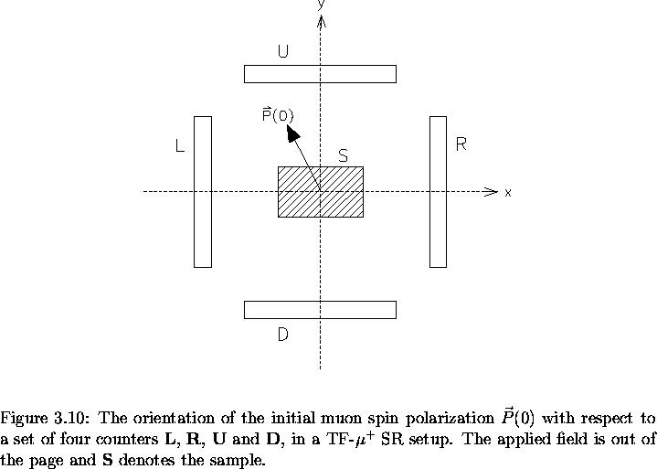
directions. A more efficient setup is the 4-counter arrangement depicted
in Fig. 3.13, where additional
counters are placed on the y and
-y axes. The L and R counters monitor the x-component
of the polarization Px(t) as before, while the U and D
counters measure the y-component of the polarization Py(t).
Ignoring geometric misalignments and differences in counter efficiency,
Py(t) differs from Px(t) only by a phase of
 .
In
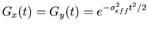
terms of the field distribution n(B), Px(t) and Py(t)are defined as:
.
In
terms of the field distribution n(B), Px(t) and Py(t)are defined as:
![\begin{displaymath}P_{x}(t) = e^{- \sigma_{eff}^{2} t^{2} /2} \int_{- \infty}^{+ \infty} n(B)
\cos \left[ \gamma_{\mu} Bt + \theta \right] dB
\end{displaymath}](img299.gif) |
(40) |
| Py(t) |
= |
![$\displaystyle e^{- \sigma_{eff}^{2} t^{2} /2}
\int_{- \infty}^{+ \infty} n(B)
\cos \left[ \gamma_{\mu} Bt + \theta - \pi /2 \right] dB$](img300.gif) |
|
| |
= |
![$\displaystyle e^{- \sigma_{eff}^{2} t^{2} /2} \int_{- \infty}^{+ \infty} n(B)
\sin \left[ \gamma_{\mu} Bt + \theta \right] dB$](img301.gif) |
(41) |
where,
 .
For an applied field in the
.
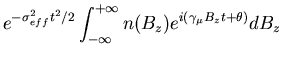
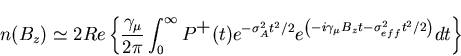
For an applied field in the  -direction, the muon spin polarization
transverse to the magnetic field Bz may be described by
the complex quantity [81]
-direction, the muon spin polarization
transverse to the magnetic field Bz may be described by
the complex quantity [81]
The real Fourier transform of the complex muon polarization
 approximates the field distribution n(Bz)
with statistical
noise due to finite counting rates
[34]. At the later times in the asymmetry spectrum, most of
the muons have already decayed. With few muons left, the statistics
at these later times are low, resulting in increased noise at the end
of the asymmetry spectrum. Using the fact that
is defined only for positive times
approximates the field distribution n(Bz)
with statistical
noise due to finite counting rates
[34]. At the later times in the asymmetry spectrum, most of
the muons have already decayed. With few muons left, the statistics
at these later times are low, resulting in increased noise at the end
of the asymmetry spectrum. Using the fact that
is defined only for positive times  ,
the field distribution
n(Bz) may be written:
,
the field distribution
n(Bz) may be written:
 |
(43) |
where the gaussian apodization parameter
 is chosen
to provide a compromise between statistical noise in the spectrum
and additional broadening of the spectrum which such a procedure introduces.
is chosen
to provide a compromise between statistical noise in the spectrum
and additional broadening of the spectrum which such a procedure introduces.
The complex asymmetry for the 4-counter setup is defined as:
where Ax(t) and Ay(t) are the real and imaginary
parts of the complex asymmetry, respectively. The number of counts
per second in the ith counter [i = R (right), L
(left), U (up) or D (down)], may be written:
![\begin{displaymath}N_{i}(t) = N_{i}^{\circ} e^{-t/ \tau_{\mu}} \left[ 1 + A_{i}(t)
\right] + B_{i}
\end{displaymath}](img317.gif) |
(45) |
where
 is the asymmetry function
for the ith raw histogram. Rearranging Eq. (3.45):
is the asymmetry function
for the ith raw histogram. Rearranging Eq. (3.45):
![\begin{displaymath}A_{i}(t) = e^{t/ \tau_{\mu}} \left[
\frac{N_{i}(t) - B_{i}}{N_{i}^{\circ}} \right] - 1
\end{displaymath}](img319.gif) |
(46) |
In terms of the individual counters depicted in Fig. 3.13,
the real asymmetry
Ax(t) and the imaginary asymmetry Ay(t) may be written:
![\begin{displaymath}A_{x}(t) = \frac{1}{2} \left[ A_{R}(t) - A_{L}(t) \right]
\end{displaymath}](img320.gif) |
(47) |
![\begin{displaymath}A_{y}(t) = \frac{1}{2} \left[ A_{U}(t) - A_{D}(t) \right]
\end{displaymath}](img321.gif) |
(48) |
In the present study, the real and imaginary parts of the asymmetry
are fit simultaneously. For the vortex state of
 ,
the real asymmetry can be fit with
Eq. (3.39). The imaginary part of the asymmetry can be fit with
the same function, but with a phase difference of
.
,
the real asymmetry can be fit with
Eq. (3.39). The imaginary part of the asymmetry can be fit with
the same function, but with a phase difference of
.
Next: The Rotating Reference Frame
Up: Measuring the penetration depth with TF-SR
Previous: Modelling The Asymmetry Spectrum of the Vortex State
Jess H. Brewer
2001-09-28