


Next: Zero-Field SR (ZF-SR)
Up: SR Spectroscopy
Previous: Transverse-Field SR (TF-SR)
Contents
A common procedure often used to visualize the internal magnetic field distribution, is to perform a fast Fourier
transform (FFT) of the muon-spin polarization function such that
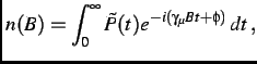 |
(3.9) |
where
 =
=
 is in general complex. However there are two limitations to the measured time
spectrum that affect the FFT. First, due to the finite lifetime of the muon, there are fewer counts at the later times.
Second, the length of the time spectrum is finite. These features introduce noise and ``ringing'' in the FFT spectrum. To
smooth out these unwanted features, one can introduce an apodization function
is in general complex. However there are two limitations to the measured time
spectrum that affect the FFT. First, due to the finite lifetime of the muon, there are fewer counts at the later times.
Second, the length of the time spectrum is finite. These features introduce noise and ``ringing'' in the FFT spectrum. To
smooth out these unwanted features, one can introduce an apodization function
 such that
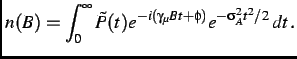 |
(3.10) |
This procedure results in a time spectrum that smoothly goes to zero at later times. However, the drawback is that this
introduces an additional source of broadening which also smooths out the the sharp features of interest. Nevertheless, FFTs
remain useful as an approximate visual illustration of the internal magnetic field distribution and for comparing the
measured  SR signal with the ``best-fit'' theory function from the time domain.
Next: Zero-Field SR (ZF-SR)
Up: SR Spectroscopy
Previous: Transverse-Field SR (TF-SR)
Contents
Jess H. Brewer
2003-07-01