The first simulation will be very simple. With the mouse, select the circle picture on the left-hand toolbar, then position a circle in the window. You position the center of the circle by clicking the mouse, which produces a standard-sized circle, along with 4 small squares. By grabbing one of the squares with the mouse you can resize the circle. Try to change the size of the circle.
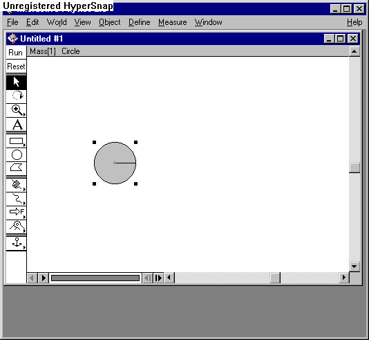
Figure: A circle object created with the default size.
We are now ready to run the simulation. Click on Run, then observe what happens. You can stop the simulation by clicking Stop, then reset it by clicking Reset.
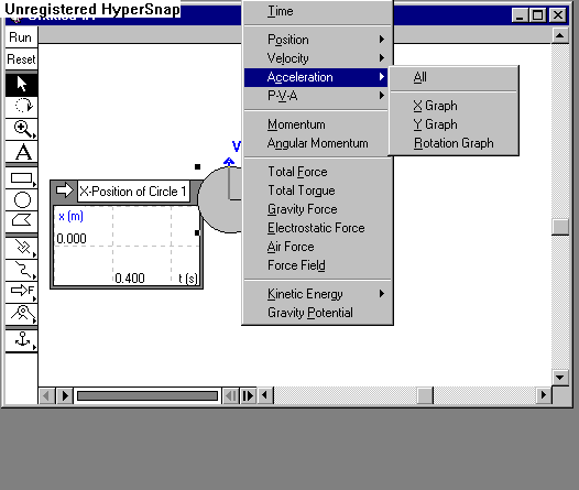
Rather than just watching the simulation, we can plot the position, velocity and acceleration of the object. First, select the object with the mouse by clicking on the object. You may need to select the Pick tool first by clicking on the arrow on the left hand toolbar. Next, pull down the Measure toolbar item, and select either Position, Velocity, Acceleration, or all three with P-V-A. You are given the choice of measuring either the x or y components of each of the quantities, or both (except for in the P-V-A graph). Try running the simulation and measuring various kinematic variables of the mass. You can change the graph appearance by clicking on the arrow on the top left corner of the measurement window. Try each of the different graph types.
You can also vary the properties of the circle you are studying. Select the circle by clicking on it, then type Alt-Enter (at the same time) which should present you with a new window entitled Properties. You can select any of the objects, forces or constraints which are defined in your simulation with the scrolling window or by clicking on that object. Available properties include the mass, velocity, moment of inertia, charge etc. You can also change the initial velocity of the object by clicking at the center of the object, then dragging the mouse in the direction you wish for the velocity vector. The length of the arrow which appears is proportional to the velocity. Vary the initial velocity of the object and observe the effects on its motion.
We can introduce several objects and allow them to interact. To illustrate this, open a new window (from the File menu item) and create a circle object with no initial velocity. Then create a poly-line or rectangular object by selecting the item on the left-hand toolbar. Draw an object underneath your circle. If you run the simulation at this point, both objects fall under gravity and never interact. We wish the fix the rectangular object: we do this by attaching an anchor to it. Select the anchor picture from the left hand toolbar and then attach it to the rectangle by placing the pointer over the object and clicking. Now try running the simulation. What happens? The simulation is designed to simulate ``real'' materials, and therefore includes effects of elasticity (the co-efficient of restitution) and friction. By selecting an object in the Properties window you can change the elasticity or friction coefficient. When a property actually depends on two objects, such as the elasticity coefficient, the simulation uses the smaller of the two for the collision. For example, if both objects have an elasticity of 0.5 the simulation will give the same results as if one were 0.5 and the other were 1.0 or 0.8. Set the elasticity coefficient of the rectangular surface to 1.0, then run the simulation for several values of the circle's elasticity between 0.5 and 0.99.
Qualitatively, what happens as you vary the elasticity?
Although you can see what is happening in the simulation while you vary parameters, it is difficult to get a clear quantitative result. We can export the results of any simulation for any variable we can measure (using a Meter in the terminology of the program) and the Export Data function of the File menu. To use this feature, set up the simulation you wish to run and run it. Then, Stop and Reset. Select the Export Data function and enter a filename when prompted. Use something like your last name and a number for the filename (e.g. Smith1) and take the default extension of .dta so that the files can be deleted later when the experiment is complete. When you complete the name and select the checked box, the results of the simulation will be written to the selected file as the simulation runs. You can then read this file with another program such as an editor (Notepad for example).
Run the simulation for a series of elasticity values between roughly 0.5 and 0.99, saving the results in a series of files. Be sure to keep track of which files contained which data as you go along (or you will end up with many unlabelled files). Do this for perhaps 5 different values of elasticity. Edit the files using the Windows Notepad editor. Draw a graph of the height reached after each bounce vs. the the number of the bounce. You can use the same graph for each of the different trials, but use different symbols for different values of elasticity.
For each file, calculate the ratio between adjacent maximum heights following each bounce. Does the maximum height decrease by a similar amount for a given value of elasticity? Calculate the average decrease in the maximum for each elasticity as well as the standard deviation in the mean (as a measure of its uncertainty) and graph it as a function of the elasticity. Note that the maximum height is proportional to the gravitational potential energy and therefore the total mechanical energy in the system. From your graph, how does the rate of mechanical energy loss depend on the elasticity of the collision?