next up previous contents
Next: 5.3 Linear Coupling; One-Phonon Up: 5 Quantum Diffusion I: Previous: 5.1 An Introduction to

5.2 Renormalization of the One-Phonon Interaction

We would like to be able to write the wave functions of the lattice with the particle present, $\Psi_m({\bf R}_i)$,in terms of the normal modes of the lattice without an interstitial. However, $\Psi_m({\bf R}_i)$ is an eigenfunction of the Hamiltonian which includes the lattice-interstitial interaction,

while the wave functions of the lattice without the interaction $\Psi_n^{(0)}$ is an eigenfunction of ${\cal H}_0$ - the Hamiltonian of the bare lattice.

By performing a transformation of the one-phonon interaction we can write these wave functions in the same basis, allowing us to evaluate the overlap,

\begin{displaymath}
\langle \Psi_n({\bf R_i}) \vert \Psi_m^{(0)} \rangle. \end{displaymath}

We define the polaron operator ${\hat \Lambda}$, a unitary operator, relating these two complete sets of wave functions by the sum
\begin{displaymath}
\Psi_m({\bf R}_i) = \sum_n \Lambda_{nm}({\bf R}_i) \Psi_n^{(0)}.\end{displaymath} (1)
The operator $\Lambda({\bf R}_i)$ here describes, in terms of the normal modes of the lattice, how the lattice wave functions change when the lattice responds to the presence of the interstitial at site ${\bf R}_i$.

Overall, the method of calculating the interstitial diffusion rate will be to describe the shifted atomic positions in both the initial and final states in terms of linear combinations of non-interacting environmental states, which include temperature-dependent numbers of phonons. The overlap between initial and final states is then given by the coefficients in these sums. Most of the following derivation will be the evaluation of the temperature dependence of these coefficients.

Fermi's Golden Rule then gives the transition rate
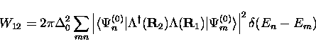
\begin{displaymath}
W_{12} = 2 \pi \Delta_0^2 \sum_{mn} 
\left \vert
 \langle \P...
 ..._1) \vert\Psi_m^{(0)} \rangle
\right \vert ^2
\delta(E_n - E_m)\end{displaymath} (2)

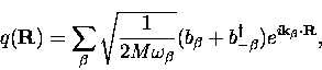
We will consider two cases of coupling to lattice excitations - corresponding to the linear and quadratic terms of a Taylor expansion of the Hamiltonian - which govern the behavior at high and low temperatures respectively. In this theory, displacements of atoms from their equilibrium positions in a harmonic potential are being written in terms of the normal modes of the lattice.

Let us first consider a very simple example to introduce the idea of writing oscillator displacement in terms of operators. In general, the Hamiltonian of a harmonic oscillator is the sum of kinetic and potential energies
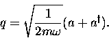
where p and q are the momentum and oscillator displacement and the raising and lowering operators are defined as

It follows that we can write the displacement of the harmonic oscillator from equilibrium, in terms of these operators,
\begin{displaymath}
q = \sqrt{\frac{1}{2 m \omega}} (a + a^{\dagger}) .\end{displaymath} (3)
Analogously, the displacement of atoms in a lattice can be written, in terms of a sum over the phonons present,
\begin{displaymath}
q({\bf R}) = \sum_{\beta} \sqrt{\frac{1}{2M\omega_{\beta}}}
...
 ... + b_{-\beta}^{\dagger}) e^{ i{\bf k}_{\beta}
 \cdot {\bf R} },\end{displaymath} (4)
in which $b_{\beta}^{\dagger}$ ($b_{\beta}$) is the operator that creates (annihilates) a phonon of frequency $\omega_{\beta}$,where ${\pm\beta} = (\pm{\bf k}, \lambda)$, the wavevector and branch index respectively.


next up previous contents
Next: 5.3 Linear Coupling; One-Phonon Up: 5 Quantum Diffusion I: Previous: 5.1 An Introduction to