Muonium Chemical Kinetics Exercise:

Mu + F₂

for TSI 2011 Data Analysis workshops

Muonium, or Mu, is like a light isotope of hydrogen with a positive muon as its nucleus, weighing only 0.114 amu. Therefore it is very attractive for studying kinetic isotope effects in chemical reactions, with extreme mass ratios of 1 : 0.114 (8.77) when compared with ¹H, or 2 : 0.114 (17.54) for ²H. Contrast this with ¹³C : ¹² C = 1.08.

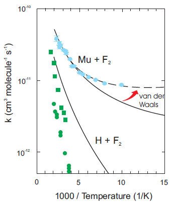
The extremely low mass of Mu gives it a long de Broglie wavelength (λ = h/p) giving increased quantum tunneling past a reaction barrier, particularly at low T (implying low p). This causes deviations from the classical Arrhenius relationship (k = A e^E_a/RT).

Muonium forms in two spin states, with the two (µ, e) spins parallel or antiparallel. Briefly, the muon spin in the parallel portion (usually called "triplet muonium") precesses in a magnetic field about 100 times faster than a bare µ⁺ or one in an all-spin-paired molecule. (See lectures.) Chemical reaction of Mu changes the magnetic/spin environment of the µ⁺ precession frequency so the products lose phase coherency with the Mu. This creates a relaxation of the Mu precession signal as the Mu is consumed.

The Experiment

The goal is to measure the temperature dependence of the chemical reaction

Mu + F₂ → MuF + F

and the exercise now is to fit some existing data to derive the rate constant at some particular temperature. In experiment 420, weak transverse-field µSR measurements were made on various mixtures of N₂ and F₂ gases at various temperatures. The quantity of F₂ was measured in a standard volume and pushed into the reaction vessel by N₂. The ratio of these two volumes is 108.1/13788.

The Exercise

Visit the TRIUMF µSR runs database at http://musr.ca/mud/runSel.html and search for Experiment 420.

Choose one of the temperatures below room temperature; preferably, different people will choose different temperatures. (A different reaction vessel was used above room temperature so you won't know the dilution factor for calculating the F₂ concentration.) Click the check-boxes for the F₂ runs at your chosen temperature and include a run of pure N₂ (zero F₂ concentration) near that temperature. (Allow pop-ups in your browser!)

Click on the run-number button for one of these runs and investigate the run header information, especially the names and ordering of the data histograms. Display the histogram data (plot button); you will probably notice that the data at the end of the time range is bad. Plot the Fourier transform (FFT button) and note the frequencies to use as initial guesses for fitting. You might also make plots for all your selected runs simultaneously, using buttons in the small Run List window.

When you know which runs you want to fit, click Zip & Download Runs at the bottom of the Run List window to bring the selected runs into your computer; then unzip the download into the directory where you want to fit them.

If you are working on bnqrexp.triumf.ca, downloading the runs is not required, as all runs are directly accessible in the /data/<beamline>/<year>/ directories on that host; unfortunately this is not available on the workstations in Hennings.

Use musrgui or (on bnqrexp.triumf.ca) physica ['t0', 'bkgd' and 'early' commands] to determine the t = 0 bin, background bin range and good data bin range. This is necessary because the values are poorly set in the data files! Checking one run should be sufficient. Prepare your fit-control template file, for either musrfit (.msr) or msrfit (.i), starting from another such file. There will be a sum of two signals, and each of those will have amplitude, exponential relaxation, and precession (frequency and phase). You should probably fit the two-counter asymmetry, in which case there is an alpha parameter. Use and modify your template to analyze each run. If you see how, collect the fit results in a .db or .csv file for further analysis. Now we hope there is still time to do something with the relaxation rates determined from the fits! The experimental reaction rate constant (for the chosen temperature) is the slope of the line fitting relaxation rate (λ_Mu, for the high frequency Mu precession) versus concentration (C) of F₂

λ_Mu = λ₀ + k_exp C_F₂

Use the ideal gas law to calculate C_F₂ for each run based on the measured pressure in the Standard Volume (check each run title, 't'=Torr). Note that the SV is at room temperature, say 295 K, not at the reaction vessel temperature! Multiply by the ratio of volumes 108.1/13788 to get the C_F₂ in the reaction vessel. Enter the concentrations in your .db or .csv results file.

Use the tool of your choice (muview, physica, oocalc, xyfit . . . ) to plot and find the slope of λ_Mu vs. C_F₂; the slope is the rate constant at your temperature. Maybe we can all combine results onto an Arrhenius plot!

Hints: Don't be tempted to force the ratio between frequencies! The two signals sample different magnetic fields and the ratio comes out wrong. Don't try any global fits; just do one run at a time. You can include or leave out a relaxation for the low-frequency signal; its relaxation is near zero. If you are stuck, template input files for run 100 are provided, 100.i and fit100.msr. These show the proper bin ranges as well as the function parametrization. 1 atm = 760 Torr. pV = nRT, R = 0.08205 (L atm)/(mol K) = 62.3637 (L Torr)/(mol K).

Muonium Kinetics - After Word

When this experiment was performed, the theoretical understanding of the potential energy surface and the reaction dynamics were claimed to be more accurate than experiment. However, the Mu data [Gonzalez et al., J. Chem. Phys. 91 (1989) 6164] clearly demonstrated a far greater contribution from quantum tunneling than was expected, going right to the limit of Wigner threshold tunneling where the reaction rate becomes independent of temperature at low T. A decade later (and another), the problem was revisited theoretically, and the conundrum resolved. See Figure 1. By accounting for the weak, long-range, van der Waals force between reactants, Takayanagi and Kurosaki [J. Phys. Chem. A101 (1997) 7098], then Tanaka and Takayanagi [Chem. Phys. Lett. 496 (2010) 248] showed that the reaction barrier was even narrower than previously thought, though not substantially lower. Performing the calculation of reaction rate after accounting for this difference gave excellent agreement with the rate constants measured by µSR at all temperatures!

Figure 1: Arrhenius plot for the H(Mu) + F₂ reaction. The green circles and squares are results of two measurements for H + F₂ (which don't agree particularly well). The cyan circles are the Mu + F₂ results. How does your fitted data point fall on this plot? Two theoretical calculations are shown, with and without the van der Waals contribution. The 2010 calculations on a new ab initio surface agree less well with the Mu results, but fit the lower H results very well. Clearly the reaction kinetics are now well understood.

Jess H. Brewer